Parallel Processing

Blending processed and unprocessed sound is a classic and effective technique that can provide drastic improvements – and it can be done in every DAW!

What is it?

The difference between processing a sound and parallel processing is simple. Both start out with an original, unaltered sound and signal path. In a processed sound, there is no amount of the original signal left. The sound passes through the processing and is altered before continuing to the output; all you hear is the processed sound. Typically this is what is done during the mixing phase. We will add EQ, compression, saturation, etc. to a sound.

Parallel processing, on the other hand, leaves the original sound unaltered but adds an amount of processed sound alongside it. It’s the blend of these two elements that constitutes the end result. Adding a reverb or delay effect is not regarded as parallel processing. Parallel processing relates more to generating a whole new sound by means of compressing, equalizing, filtering, distorting, re-amping, and generally using and abusing non time-based audio processors.

Parallel processing is a non-destructive technique. The basic process is done this way: the original sound is on one channel. An auxiliary input track is created next to it, leaving us now with two tracks. On the 2nd track we add whatever effect we want to use, i.e. a distortion effect plugin. Using a bus send on the original track, send this to the new auxiliary track with distortion. You can add a lot of distortion if you want! The channel fader for the aux track will most likely not be at unity (0). While playback is engaged, starting with the fader down all the way at infinity, slowly bring up the fader on the aux track until the distortion is heard. Set the fader where it suits you. Doing things this way allows the original signal to go to the main output, and then the parallel distorted signal is also being sent to the main output, but only the amount we desire to have. Blend these two tracks to taste.

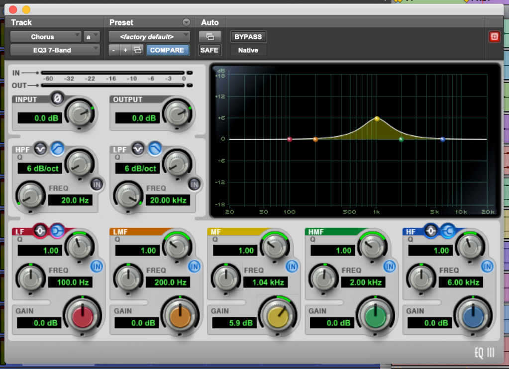
In the screenshots below there is a synth bass track that wasn’t coming through the mix very well. It has a lot of energy below 100 Hz. To help bring it out in the mix better I added some distortion using parallel processing. On the original bass track I added a bus send (bus 1), routing it to a mono aux. track which has the distortion plugin.

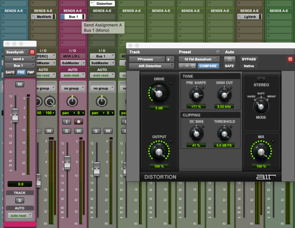
Notice that on the bus send I set it to pre-fader send and that the volume fader is set to unity (0). It just so happens that on the aux channel that has the distortion plugin, the channel fader is set quite high, -5 dB or so. Because of the type of preset I used on the distortion plugin I could get away with this strong of a mix level. Usually when doing parallel processing the channel fader is much lower. I did start with it all the way down, though, and brought it up slowly until it made a difference in the mix to my liking.

In the next screenshot I am using a saturation plugin. This is adding some harmonics which will emulate some analog equipment.

Again, because of the type of processing I am doing, some of the settings are a little different from “normal” use. I have never set the saturation to 1.0, but because I am using it in a parallel situation I can get away with that. Many times I will put a saturation plugin directly on a track. When I do it this way, the saturation is set no higher than .4. And again, notice that the aux channel level is set to unity. Again, because what I trying to achieve, this was acceptable.

The next screenshot is the same thing but this time I am using a compressor. This is, of course, known as parallel compression.

All settings for I/O routing are the same. Notice on the compressor I am achieving 6 dB of gain reduction, while also adding 6 dB of makeup gain. The 6 dB gain reduction is almost an arbitrary number. I knew since I was doing parallel processing I could afford to hit the compressor a bit harder, thus 6:1 ratio with 6 dB GR. Remember, I can always “dial in” the amount of the compressed signal I desire alongside the unprocessed signal.

While listening through earbuds, all 3 of these effects of parallel processing worked really quite well (saturation, harmonics, compression). The goal was to get the sub-bass synth bass to come through the mix better. This was definitely achieved with great results.

On a rap track I’m currently mixing I used parallel processing on the hook lead vocal. I set up a compressor on one aux. channel, and a doubler plugin on a 2nd aux. track. I then sent two different bus sends from the original vocal track to each of these two aux. tracks (pre-fader, unity send). Each aux. channel fader was then set appropriately. In this case, they were not at unity. The doubler track was set somewhere near -20 or -30 dB. The compressor track was also set close to the same.

Parallel processing is a great tool to use and one of many in any mixer’s toolbox. You are only limited by your imagination! I read about one of the top mixers who uses parallel processing even for EQ. He prefers not to EQ the original track, instead preferring to do it with a parallel track. Many times we don’t want to alter the original track to drastically, but still add an effect. This is a perfect scenario for parallel processing!

I hope you find this information helpful!

And …… HEY! Make it a great day!

Tim

EQ – Different Frequency Bands [20 Hz – 20 kHz]

Learning what different frequencies sound like and the effect they have on the sound of different instruments is an invaluable skill. These are the names we use to classify the bands – the frequencies are approximate, so use your ears!

> 20 – 60 Hz – Sub-Bass: Gives boom, depth, and richness – too much sounds flabby and out of control. Small speakers don’t reproduce this.

> 60 – 150 Hz – Bass: ‘Thump’ and punch in drums, especially kick and snare, and richness in bass and guitars. Too much sounds woolly.

> 150 – 1 kHz – Lower mid: Important for warmth, but too much sounds thick and congested. The 500 Hz – 1 kHz region especially is crucial for a natural vocal tone, but too much sounds boxy and nasal.

> 1 – 3 kHz – Upper mid: The most sensitive area of the ear, important for edge, clarity and bite, but too much will sound harsh and tinny.

> 3 – 8 kHz – Low Top: Provides fizz and sizzle; and edge and aggression in guitars – too much sounds thin and brittle.

> 8 – 12 kHz – Top: Gives openness, air and clarity – too much sounds over-bright and glassy.

> 12 – 18 kHz – Very high top: These frequencies can add sheen and sparkle and sweeten things up, but too much sounds unnatural, gritty and forced. [FYI – I have the Kush Clariphonic parallel EQ hardware. I add these frequencies on my mixbuss or sometimes use it for vocals. It really opens up that top end. A little goes a long way.]

Tip #1: Don’t solo an instrument when EQ’ing. Set the EQ when playing the instrument in context with the rest of the track. You can solo to quickly check things, but be sure to take out of solo mode fairly quick.

Tip #2: Sometimes when soloing a track or instrument, the EQ we add makes that instrument sound worse! But in context of the whole mix it sounds great. That is what matters. Part of the time you can expect this to happen.

Tip #3: If there are two parts that are fighting in the mix because they occupy the same frequency range, it can sometimes help to boost the EQ on one of them and cut the other at the same frequency, then reverse the strategy and boost the second sound in a different place while cutting the first. This emphasizes the contrast between the two parts, with gentler boosts, and helps stop things sounding unnatural.

Tip #4: In regard to Tip #3 above, this can sometimes be called ‘masking.’ Masking is when two instruments are fighting for the same frequency or frequency space. For example, kick and bass guitar. If when the kick hits, the bass is obscured some, this is masking. Using Tip #3 above will help get rid of this problem. Make sure to ‘cross-EQ’ both ways. In other words, boost instrument 1 and cut instrument 2 in same place. Then boost instrument 2 and cut instrument 1 in same place.

Tip #5: Do a ‘boost & sweep.’ When searching for a frequency that you want to get rid of, use a bell curve EQ (band, or parametric), boost @12 dB with a somewhat narrow bandwidth (high Q). Sweep up and down in frequency until you find (hear) the unwanted or annoying frequency. Then set that band for a cut instead of a boost. How much you cut depends on the specific situation, it might be a little or a lot.

As always – I hope this helps!

And ……. HEY! Make it a great day!

T

The Different EQ bands and What they mean

Throughout my blog series on EQs I am going to refer to the free EQ plugin that comes with Pro Tools, the Digirack EQ III 7-band. First, let’s talk about the input/output LED meters and gain controls (top left of the plugin). This simply shows the input and output signal level running through the EQ. Always check to make sure there is no clipping going on. If on the input or output side the signal is clipping, hitting red, simply turn the respective gain knob down until there is no longer any clipping happening. It is normal to adjust these gain knobs. With the input gain knob is a symbol, Ø. This is the polarity switch “button.” This will invert the phase of the incoming signal. If you don’t know what this is, I will cover it in a later post. It’s a little more advanced, but easy to understand and know when to use. For now, it won’t concern us.

Just beneath the input/output section are two filters. There is a high pass filter and low pass filter (HPF, LPF).

High Pass Filter

Low Pass Filter

There is also a notch filter. It looks like a line with a ‘V’ in the middle of it. (I couldn’t find a pic of one.)

-∨- (notch filter)

The high pass filter alllows high frequencies to pass through the EQ, while cutting low frequencies, not allowing them to go through the EQ. Conversely, the low pass filter allows low frequencies to pass through and cuts high frequencies. The notch filter takes a small section of audio and makes a deep cut (-12 dB or more). It takes a “notch” out of a small section of audio frequencies. The frequency can be set by the user. One use for the notch filter is for plosives on a vocal track. When a vocalist pops, say a ‘p,’ set the notch filter at 100 Hz. It should diminish it greatly or make it go away completely. You may have to sweep the EQ up or down a little to take care of it.

The two filters each have an “IN” button to engage them. They will light up blue when engaged. The frequency, of course, can be set to whatever you want.

Lastly, there is a setting that is used for the HPF/LPFs that tells the filter how steep of a cutoff you want. If we are allowing high frequencies to pass through and cut out low frequencies, how strong do we want to cut off those low frequencies? The slope is set per octave. The setting choices are 6 dB per octave, 12 dB/oct, 18 dB/oct, and 24 dB/oct. As an example, let’s say I set a high pass filter at 200 Hz, with a 12 dB/octave slope. What this means is that only frequencies above 200 Hz will pass through the EQ (and anything further in the signal chain), and frequencies one octave down (100 Hz, remember from my previous post?), will be 12 dB quieter. Another octave down, 50 Hz it will be another 12 dB quieter. There are times we want a steep cutoff, like 24 dB/octave and other times when we might want 6 dB/octave.

Look on the left side of the GUI window, which shows the graphic interface. There are small numbers. On the center line is 0. This is where all EQ bands start. In out example, since we’re cutting at 200 Hz, at 100 Hz the downward slope will be at -12 dB. At 50 Hz it will be -24 dB.

I hope this hasn’t been too confusing. Try experimenting with these filters on a mix you’re working on. Keep your ears open when doing this. You can even experiment on a piano or acoustic guitar track. Set the HPF up higher, like 400, 500 Hz. Change the different octave settings. You should hear what’s happening.

As always,

Make it a GREAT day!

Tim

EQ Overview and Introduction

In the next series of blog posts, I’m going to go through EQ, or equalization. I will talk about why we use it, and when and how to use it. I think EQ is easier to understand than compression (my last series of blog posts), but when I see EQs added by young producers and engineers, I realize they are just as lost using EQ as a compressor. Partly, this is because they don’t understand frequencies.

In this blog I am going to start with an overview. I think to understand EQ and use it properly, one must understand frequencies, our ear’s perception to frequencies, the frequency spectrum (or range), and frequency specifics of individual instruments.

To start with, the ear hears 20 Hz to 20,000 Hz (or 20 kHz). This is, of course, ideal, but starts to become less (mostly on the high end), soon after we’re born. If you’re serious about a career in music, it would serve you well to NOT listen to loud sources for very long. Personally, I wear ear protection when using my leaf blower and shop vac!

If you think about an acoustic piano, the lowest note is A0, 27.50 Hz, and the highest note is C8, 4186 Hz. I bring this up because I think it helps us equate pitch with frequency. Next chance you get, go play specific notes on a piano (acoustic or digital), and then consult a chart as to the frequency of that note. For instance “middle” C is 262 Hz. A440 (the A just above middle C) is 440 Hz.

Do you know what an octave is? An octave, at least on a piano, is from, say, middle C up or down to the next C. This happens to be 8 white keys, thus octave. Using octaves, the frequency either doubles (up an octave) or halves (down an octave). So middle C (C4), 262 Hz, up an octave goes to C5, 523 Hz. (Technically, C4 is 261.63 and C5 is 523.25 Hz.) The A above middle C, A4 is 440 Hz. Up an octave is 880, down an octave is 220. Down another octave is 110, then 55, then 27.50, the lowest note on the piano. All instruments, of course, can go up or down octaves at a time.

The lowest note on a guitar is E2, 82 Hz. Guess what a bass guitar’s lowest note is? One octave down, 41 Hz. This is important. For one reason, when EQing either of these instruments, I know there is no useable information below those frequencies, so I will use a high pass filter set just below those frequencies. This helps to clean up the sound of these instruments, make them less muddy.

The frequency spectrum (20 Hz – 20 kHz) is broken into ten octaves:

1. 20 – 40
2. 40 – 80
3. 80 – 160
4. 160 – 320
5. 320 – 640
6. 640 – 1280
7. 1280 – 2560
8. 2560 = 5120
9. 5120 – 10, 240
10. 10,240 – 20, 480

So, the lowest note on a bass guitar, 41 Hz is in octave 2; lowest guitar string is octave 3; middle C on piano is octave 4; A440 is in octave 5. Where do vocals sit? Fullness, for example, is 140 – 440, octave 3 to 5.

A different and more effective way to think about the frequency range is to break it up into five broader ranges:

1. 20 – 100         Bass (Sub Bass)
2. 100 – 500       Mid Bass (Upper Bass)
3. 500 – 2 kHz   Mid Range
4. 2 k – 8 kHz    Upper Mid Range
5. 8 k – 20 kHz  High (Treble)

Bass:                           Depth, Power, Thump

Upper Bass:              Warmth, Body, Fullness

Mid Range:               Bang, Nasality, Horn-like, Fullness of high notes

Upper Mid Range:  Presence, Edge, Punch, Brightness, Definition, Excitement

Treble:                        Brilliance, Sizzle, Treble, Crispness, Airiness, Breathiness

As example, electric guitar has too much “edge,” cut in the upper mid region. Vocal sounds a little nasal, cut in mid range area. The overall track needs more power and punch, boost bass region.

————————–

To go deeper, the human ear (and mind) hears and perceives sound differently at different frequencies and levels of loudness. Generally speaking, we are more sensitive to mid range and upper mid range frequencies. The ear is less sensitive to low frequencies at lower volumes, and slightly less sensitive to higher frequencies compared to mid range frequencies at the same volume. Being more sensitive means we hear it easier and more readily.

Another way to say this is at low listening volume, mid range frequencies sound more prominent, while the low and high frequency ranges seem to fall into the background. Conversely, at high listening volumes, the lows and highs sound more prominent, while the mid range seems comparatively softer. Confusing? Yes. But extremely important to understand.

To illustrate – Let’s say you’re working on the EQ of a mix, and as you listen back at low levels, you think the lows and highs could use a boost. So you boost them, and it sounds great. The next day you listen back at a high volume, and notice the lows and highs are too loud, so you cut them back down some. Sound familiar? This is the Equal Loudness Contour effect.

There are two different charts one could consult to dig deeper into this important, albeit nerdy and technical subject – Fletcher-Munson Curves and Equal Loudness Contour. There are many articles available online regarding these two subjects, so I will not get into them. BUT, it is extremely important to realize how important these affect your work as an audio professional!

I went a little more in depth than normal in this post, but I hope it helps you to understand what is involved when learning to become an successful producer or audio engineer.

Peace –

And, HEY! Make it a GREAT day!!

Tim

EQ – General Use (Tips/Tricks) (Part 3)

Avid Pro Tools Dyn3 7-band EQ (free plugin)

Understanding the overall structure of the EQ landscape is important to properly EQ individual tracks and to get them to fit nicely in the full mix. There are certain EQs out today that show the frequency band inside the EQ GUI. These can be quite helpful. Many EQs don’t have this feature. In either case, it is important to have a good understanding of essential frequencies for each instrument along with a fuller understanding of the overall spectrum.

If boosting a frequency band (using a bell curve), be conservative. Try to only boost 1, 2, or 3 dB. Don’t do anything crazy like a 6 or 10 dB boost. Also, when boosting, use a wide Q, which is a low Q number. Try starting with 1, or even less than 1. This type of a boost sounds more natural, as if the frequency is really there in the instrument or the recording if the instrument. This is seen below with the MF band using a 2.6 dB boost and a .84 Q setting.

Gentle boost with wide Q setting

Another tip is when cutting, use a narrow bandwidth, high Q setting. This can be seen below with the MF band. Notice the 2.54 Q setting.

EQ cut using narrow, or high Q, setting

We use a narrow bandwidth when cutting, so as to not affect too many frequencies. Usually we cut to take out annoying frequencies. If the bandwidth is too wide (cutting out a lot of frequencies), it will make the instrument sound unnatural.

This next one falls outside the context of our ‘Q’ setting discussion but is a really good idea. Use a HPF (high pass filter) on the low end to cut out unwanted or unneeded frequencies. Many instruments, including voice, don’t use frequencies below 100 Hz. Use a filter to take these out. It will clean up the track or instrument helping it to not sound so muddy.

HPF at 100 Hz

Try setting the frequency around 100 Hz. This will take out many unused or unwanted frequencies making the track “cleaner” sounding.

Starting with these three simple rules will help your tracks and mixes sound better, cleaner (not muddy) and more natural.

As always, Make it a GREAT day!!

Tim

What is the ‘Q’ setting on an EQ?

Today I am going to talk about the Q parameter on the bands of an EQ. We will be going a little deeper than we normally do, but that’s the nature of the Q factor.

The Q setting is going to affect the bandwidth of an EQ band. This means how much or how little of the frequencies will be affected with a boost or a cut. [Q stands for Quality factor]

On a basic level, one can see that when changing the Q setting, the bandwidth either gets wider or more narrow. Why does it do this, what does that affect, and how do I know which setting to use? Keep reading.

1 kHz bell curve boost

This typical view (above) is often referred to as a ‘bell’ curve due to the upper portion’s resemblance to the shape of a bell. In regard to the bell curve above, it has a center frequency of 1 kHz and a boost of 12 dB. (The solid line represents a boost; the dashed line shows if it were a cut).

The Q parameter controls the shape of the EQ curve. High Q values use steeper curves, which affect a smaller range and allow you to pinpoint specific frequencies. Low Q values affect a wider range of frequencies and tend to sound more gentle when used subtly. Q is the ratio of center frequency to bandwidth, and if the center frequency is fixed, then bandwidth is inversely proportional to Q—meaning that as you raise the Q, you narrow the bandwidth, and when you lower the Q, you widen the bandwidth. Q is by far the most useful tool an EQ offers, allowing you to attenuate or boost a very narrow or wide range of frequencies within each EQ band. (More on bandwidth below)

When using EQs, we are concerned with how much of the bandwidth we are affecting. We do this in octaves. When dealing with frequencies (Hertz), a doubling of the number is raising one octave higher. Conversely, halving the number is lowering one octave. Middle C (on a piano) is roughly 262 Hz. Going up one octave higher, to the next C up on the piano, the frequency is twice that, or 524 Hz. Going to the C below middle C is 131 Hz.

In order to understand Q, we have to focus on two other details. The center frequency (the one we choose for the band, i.e. 1,000 Hz), also known as f₀ , and the bandwidth (f₂ – f₁).

Looking at the graph below, we see a boost of 12 dB. But we measure the bandwidth 3 dB down from 12 dB, which is 9 dB. The width of this, measured in octaves, is what the Q sets. In our example above, if the center frequency is 1 kHz, we can set the Q to affect one octave, centered around 1 kHz. Or, 2 octaves, 1/2 octave, 1/3 octave, etc. [Remember, the bandwidth is always measured at 3 dB down from center frequency]

Fig. 2

Q is defined as: Q = center frequency ÷ bandwidth

For example, a filter centered at 1000 Hz that is 1/3-octave wide has frequencies located at 891 Hz and 1123 Hz respectively, yielding a bandwidth of 232 Hz. Q, therefore, is 1000 Hz divided by 232 Hz, or 4.31. (Again, remember, this is 3 dB down from center frequency).

If you want to do a quick estimate of bandwidth, take the inverse of the Q number. A Q of 1 will refer to a one-octave bandwidth; a Q of 4 will be 1/4 octave; a Q of 2 will be 1/2 octave; a Q of 10 will be 1/10 of an octave. A Q of .25 would indicate a four-octave bandwidth. This will not give you a precise bandwidth, but will be close. The math behind these shortcuts is complicated.  It’s a relatively complex multi-step algebraic formula that ties Q and the bandwidth together. 

We can always refer to a table or chart for more precise numbers. The following table shows the frequencies of a Q setting for one-octave bandwidth (a Q setting of 1). Listed is the center frequency (which we set), along with the upper and lower frequency, for a one octave bandwidth.

Octave Bands

Lower Band Limit (Hz)	Center Frequency	Upper Band Limit (Hz)
11	16	22
22	31.5	44
44	63	88
88	125	177
177	250	355
355	500	710
710	1,000	1420
1420	2,000	2840
2840	4,000	5680
5680	8,000	11360
11360	16,000	22720

Q settings and their associated bandwidth (BW) in octaves.

Conversion chart or table ‘bandwidth in octaves’  to quality factor Q

BW in octaves	Filter  Q		BW in octaves	Filter  Q		BW in octaves	Filter  Q		BW in octaves	Filter  Q
1/80	115.4		1	1.41		4	0.267		7	0.089
1/60	86.6		1 1/4	1.12		4 1/4	0.242		7 1/4	0.082
1/50	72.1		1 1/3	1.04		4 1/3	0.234		7 1/3	0.079
1/40	57.7		1 1/2	0.92		4 1/2	0.220		7 1/2	0.075
1/30	43.3		1 2/3	0.82		4 2/3	0.207		7 2/3	0.071
1/25	36.1		1 3/4	0.78		4 3/4	0.200		7 3/4	0.068
1/20	28.9		2	0.67		5	0.182		8	0.063
1/16	23.1		2 1/4	0.58		5 1/4	0.166		8 1/4	0.058
1/12	17.3		2 1/3	0.56		5 1/3	0.161		8 1/3	0.056
1/10	14.4		2 1/2	0.51		5 1/2	0.152		8 1/2	0.053
1/8	11.5		2 2/3	0.47		5 2/3	0.143		8 2/3	0.050
1/6	8.65		2 3/4	0.45		5 3/4	0.139		8 3/4	0.048
1/5	7.20		3	0.40		6	0.127		9	0.044
1/4	5.76		3 1/4	0.36		6 1/4	0.116		9 1/4	0.041
1/3	4.32		3 1/3	0.35		6 1/3	0.113		9 1/3	0.039
1/2	2.87		3 1/2	0.33		6 1/2	0.106		9 1/2	0.037
2/3	2.14		3 2/3	0.30		6 2/3	0.100		9 2/3	0.035
3/4	1.90		3 3/4	0.29		6 3/4	0.097		9 3/4	0.034
									10	0.031

Here is yet another chart for select octave bandwidths.

Q factor as a function of the bandwidth in octaves

Bandwidth in octaves	Filter Q factor
3.0 wide	0.404 low
2.0	0.667
1.5	0.920
1.0	1.414
2/3	2.145
1/2	2.871
1/3	4.318
1/6	8.651
1/12 small	17.310 high

Below are some pictures using fabfilter’s Pro-Q with different Q settings.  Sometimes pictures explain things easier. Hopefully this will show what I’ve tried to explain with words and calculations.

2 Octave Bandwidth: Q = .667

1 Octave Bandwidth: Q = 1.414

1/2 Octave Bandwidth: Q = 2.871

1/3 Octave Bandwidth: Q = 4.36

Alternative to Memorizing These Shortcuts:

Memorizing all of the numbers above is a bit of a task.  Here is a way to calculate these Q’s simply.  It’s certainly not perfect, but it does offer a way to find these Q’s quickly.

By multiplying the number 2.05  with the first Q setting, .667 (2 octave bandwidth), you get 1.37.  When rounded up, this equates to 1.4 – a number very similar to the Q setting for 1 octave.

If you continue multiplying 2.05 by each number that comes after, you’ll be able to equate Q’s that are very closely related to the exact numbers above.

For example: 1.37 x 2.05 = 2.8 or roughly a 1/2 octave bandwidth

          2.8 x 2.05 = 5.75 or roughly a 1/4 octave bandwidth

The numbers certainly aren’t exact, but they get you close enough to a workable number, all while having you memorize only 2 numbers – .667 and 2.05.

Personally, I don’t like this because to get to a 1/4 octave, you have to run the calculation 4 times. But if this works for you – go for it!

Conclusion:

Practically speaking, setting your Q and it’s bandwidth to an octave or an octave based setting, drastically increases the musicality of your mix.  On wider settings it makes it sound more natural and musical, on narrow settings it allows you to know the notes that you are affecting. 

Consider using these shortcuts and octave based equalization whenever you want a quick, and accurate way to affect your mix.

I hope you were able to hang in there for this whole discussion. If you got lost in any of this, continue to hit it again and again until you fully understand it. I had to. Go down the rabbit hole and chase this until you “get it!”

As always, I hope this helps!

And HEY! Make it a GREAT day!!

T

The Different EQ bands and What they mean (part 2)

Dyn3 7-band EQ (Avid Pro Tools free plugin)

If you look toward the bottom of the EQ pictured above, you will notice 5 different bands: 1. LF, low frequency, red; 2. LMF, low-mid frequency, orange; 3. MF, mid frequency, yellow; 4. HMF, high-mid frequency, green; 5. HF, high frequency, blue.

In today’s blog I will talk about these five bands. I want to start with band 1 and 5. These are typically used and referred to as “shelves.” Band 1, low frequencies, is the low shelf, and band 5, high frequencies, is the high shelf.

But these two bands each have two different settings. The small left icon, next to the LF and HF, is called a bell-type EQ. It kind of looks like -o-. This will either boost or cut a section of frequencies set by you with the frequency knob. The ‘Q’ knob will determine how wide or narrow the bell curve will be. A low Q setting will give you a wide band of frequencies, and a high Q will render a narrow band of frequencies. A good rule of thumb is wide when boosting and narrow when cutting.

The typical use for this is to, say, boost the lower frequencies to bring out a kick drum or synth bass. On the high end, with the HF knob, we can boost upper ‘air’ frequencies to make guitars or vocals stand out or sound brighter. Of course, we can also cut in these frequency ranges as well.

The other icon setting is called a ‘shelf.’ This is the more common use for these two bands. Typically we use a boost here (low or high). When boosted, it looks just like a “shelf.” If on the low shelf, we set the frequency knob to 125 Hz, then everything from 125 on down (to 20 Hz) is boosted the same amount. On the high shelf, we might add a shelf for vocals starting at 6 kHz. In this case everything from 6 k up will have a boost. Of course, we can also cut using a shelf, but this happens less often then a boost.

The Q factor is a bit more complicated and will have to be reserved for another post.

Bands 2, 3 and 4 allow for bell curve settings only. These are the same as the bell curves on bands 1 and 5. These are used for low-mid, mid, and high-mid frequencies. There are only three knobs: Frequency, Gain and Q. Frequency, of course, sets the frequency that you want to work with. Gain is volume (loudness) and can be plus (positive) or minus (negative). We might say boost 2 kHz 2 dB (2 dB) which is a positive gain. Or cut 1200 Hz 3 dB (-3 dB) which would be a negative gain.

As stated above, Q determines the amount of frequencies being altered by the EQ.

As always, I hope this helps!

And, HEY! Make it a Great day!

Tim

Compression Dos & Don’ts

To wrap things up regarding compressors, I will offer 3 Dos and Don’ts as my final word for now. These are things to always keep in mind when working with compressors. Some may have been previously stated in an earlier blog post.

DO          Avoid using extreme settings to begin with, if you are just trying to control the dynamics.

DON’T   Add compression to every channel by default. Start off with minimal compression, and carefully choose where to add compressors.

DO         Experiment with different types of compressors – hardware and software. There can be differences in how they sound. Compressors can and do sometimes sound different from one another.

DON’T  Forget to bypass the compressor occasionally while setting to check the results.

DO         Remember to balance the output gain so the level doesn’t change when engaged and bypassed. This way you can accurately compare before and after. Also, typically compression is added AFTER the mix has been balanced. So you don’t want to alter levels with either compression or EQ.

DON’T  Be afraid to experiment. Some of the greatest sounds in the history of recorded music came from misused and abused compressors.

Compressors – What is the Knee and What does it do?

As you get better with compressors, you will start playing with other knobs and features. One of these is the knee. The knee refers to when and how the ratio starts to change when the compressor starts to take effect. A ‘hard knee’ means the compression becomes immediately active as soon as the input signal hits the threshold. A ‘soft knee’ means the compression becomes audible more gradually. A ‘soft knee’ also means that gentle compression starts happening further below the threshold. Another way to say this is it starts acting before the signal actuall reaches the threshold setting.

Both hard- and soft-knee compression have their uses; two examples: if you want to squash a signal’s transients quickly, you’ll want hard knee compression. If you want to use a compressor to gently glue a mix together by tightening up transients, you’ll want a soft-knee compressor.

Lastly, if you have a compressor, like the Dyn3 Compressor/limiter which comes free with Pro Tools, look at the picture of the knee. It actually looks like a human knee!

As always – I hope this helps!

And…. HEY! Make it a great day!

Tim

Compressors 201 – Threshold

A compressor has a lot of knobs and settings. They can be confusing at first. In this blog I am going to talk about one of those knobs – Threshold.

A compressor is an automatic volume control. We try to make the signal somewhat the same, static. Without a compressor, we would have to do it manually, turning the signal down, then up, then down, etc. But with a compressor, it can do that job for us.

When a signal gets loud (and crosses the threshold), it turns it down. If there’s any makeup gain, it will turn the softer signals up making them louder (along with everything else, of course).

The threshold setting tells the compressor when to start working. Put a compressor on, say, a vocal track. Pay attention to the input signal on the compressor. Let’s say the input signal is -10 dB. Now set the threshold knob to -16 dB, and the Ratio 2:1. What we’re telling the compressor to do is this: Any signal that is stronger than -16 dB, I want it to compress (lower) the signal. When the signal crosses the threshold it will get cut (attenuated) in a 2 to 1 ratio. So in this scenario, the signal is coming in at -10, with the threshold set to -16 and a 2:1 ratio. This means 6 dB is going to get compressed in a 2:1 ratio. The signal will get cut down to 3 dB over. You can think 2 becomes 1, 4 becomes 2, 6 becomes 3, etc.

If the ratio was 10:1, the signal would get compressed more. The higher the number, the more the compression. If the signal crossed the threshold by 10 dB, then it would be reduced to 1 dB.

The threshold determines how much of the signal the compressor is going to affect. You can change where the threshold is set usually in two ways. Using the Dyn3 compressor/limiter, grab the orange arrow on the signal led and slide up or down. Or to the far right at the bottom, grab the threshold knob and set up or down.

TIP: If Pro Tools is your DAW, use the Dyn3 Compressor/Limiter (free). It helps to make understanding what and how a compressor works easier.

I hope this helps!

and HEY! Make it a great day!

Tim